Introduction to Anomaly Detection

Anomaly Detection (a.k.a Outlier Detection) is a process of detecting unexpected observations in specified datasets.

Anomaly detection has two basic assumptions:

• Anomalies only occur very rarely in the data;
• Their features differ from the normal instances significantly.
  (Susan Li, 2019)

Different anomaly detection approaches shall be applied based on the characteristics of dataset and the purpose of the analysis. There are mainly two ways to deal with outliers in statistics and machine learning, namely unsupervised learning and supervised learning. Also the algorithms often been modified and integrated with other techniques to achieve specific goals in production environment, for example time series analysis.

Statistical Models

3 Sigma Rule

For one dimension outlier detection we can simply use the $3\sigma$-Rule.

Given the dataset $X = \lbrace x_1,x_2,...,x_n \rbrace$, if $X$ follows normal distribution, then its probability density function is:

$p(x,\mu,\sigma^2)=\frac{1}{\sqrt{2\pi}\sigma}e^{-\frac{1}{2}(\frac{x-\mu}{\sigma})^2}$

from maximal likelihood, we know that:

$\hat{\mu}=\overline{x}=\frac{\sum_{i=1}^{n} x_{i}}{n}$

$\hat{\sigma}^2=\frac{\sum_{i=1}^{n} (x_{i}-\overline{x})^2}{n}$

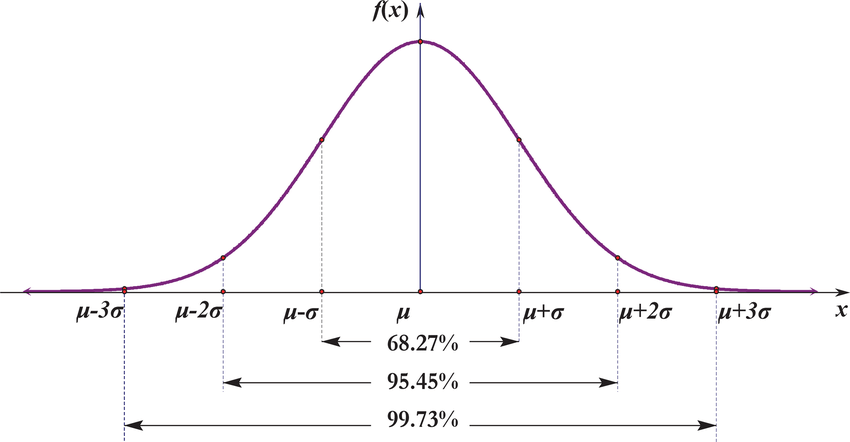
Then we create a $\mu \pm 3\sigma$ window contains 99.73% of the data. If a new point falls outside of the window (i.e. $x_k \notin (\hat{\mu}-3\hat{\sigma},\hat{\mu}+3\hat{\sigma})$), then such new data point can be perceived as an outlier.

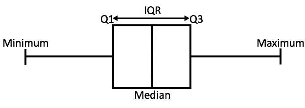
Boxlot

The boxplot can be applied to any form of distribution of the data. The define the boundary of the outlier detection, we first find the Q1 and Q3 then calculate the Interquartile Range (IQR = Q3 - Q1). The 2 outlier boundaries then defines as: $ Q1- \lambda * IQR $, $ Q3+\lambda * IQR $. (usually we take $\lambda = 1.5$ )

There are many other statistical models could perform the tasks of anomaly detection. I will probably introduce those in future posts.

Distance Based Models

Angle-Based Outlier Detection

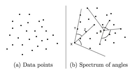
Angle-Based model is not suitable for large datasets. But it is a basic way to detect outliers by simply comparing the angles between pairs of distance vectors to other points.

Nearest Neighbour Approaches

For each data point $x_i$, compute the distance to the $k$-th nerest neighbour $d_{k}(x_i)$. Then for all data points, we diagnose the outliers are the points that have the larger distance. Therefore, the outliers are located in the more sparse neighbourhoods. However, this methods is not suitable for dataset that have modes with low density.

Local Outlier Factor (LOF)

The LOF score is equal to ratio of average local density of the $k$ nearest neighbours of the instance and the local density of the data instance itself.

Connectivity Outlier Factor (COF)

Outliers are points $p$ where average chaining distance $ac$-$dist_{kNN(p)}(p)$ is larger than the average chaining distance ($ac$-$dist$) of their $k$-nearest neighbourhood $kNN(p)$.

COF identifies outliers as points whose neighourhoods are sparser than the neighbourhoods of their neighbours.

Linear Models

Principal Componenet Analysis

I will not try to explain what PCA is in here. The major argument here is that since the variances of the transformed data along the eigenvectors with small eigenvalues are low, significant deviations of the transformed data from the mean values along these directions may represent outliers.

Let $R$ be a $p \times p$ sample correlation matrix computed from $n$ observations on each of $p$ random variables $X_1,...,X_p$. If $(\lambda_1,e_1),...,(\lambda_p,e_p)$ are the $p$ eigenvalue-eigenvector pairs of $R$, $\lambda_1 \geq ... \geq \lambda_p \geq 0$, then the $i$-th sample principal component of an observation vector $\pmb{x} = (x_1,...,x_p)$ is

$y_{i} = < \pmb{e}\_i,\pmb{z} > = \sum_{k=1}^{p} e_{ik} \cdot z_k \quad \text{for i = 1,2,...,p}$

where $e_i = (e_{i1},...,e_{ip})^{T}$ is the $i$-th eigenvector. That means

$\pmb{y} = (y_1,...,y_p)^{T} = (e_{i1},...,e_{ip})^{T}\pmb{z}$

is the principal component of vector $\pmb{x}$.

$\pmb{z} = (z_1,...,z_p)^{T}$ is the vector of standardized observations defined as

$z_k = \frac{x_k - \overline{x}\_k}{\sqrt{s_{kk}}} \quad \text{k=1,...,p}$

where $ \overline{x}_{k} $ and $ s_{kk} $ are the sample mean and the sample variance of the variable $X_k$.

Consider the sample principal components $y_1,...,y_p$ of and observation $\pmb{x}$. The sum of the squares of the standardized principal component values

$Score(\pmb{x}) = \sum_{i=1}^{p} \frac{y_{i}^2}{\lambda_i} = \frac{y_{1}^2}{\lambda_1} + \cdots + \frac{y_{p}^2}{\lambda_p}$

is equivalent to the Mahalanobis distance of the observation $\pmb{x}$ from the mean of the sample. An observation is outlier if fro a given significance level

$\sum_{i=1}^{p} \frac{y_{i}^{2}}{\lambda_{i}}>\chi_{q}^{2} (\alpha) \quad \text { where } 1 \leq q \leq p$

Non-linear Models

Replicator Neural Networks

The RNN in here is not referring the commonly known Recurrent Neural Networks. The Replicator Neural Networks, or autoencoders, are multi-layer feed-forward neural networks.

The input and output layers have the same number of nodes. Then the network is trained to learn identifying-mapping from inputs to outputs. Given a trained RNN, the reconstruction error is used as the outlier score: test instances incurring a high reconstruction error are considered outliers.

Summaries

• Staistical Methods based OD
  • Normal data instances occur in high probability regions of a stochastic model, while anomalies occur in the low probability regions of the stochastic model.
• Classification based OD
  • A classifier that can distinguish between normal and anomalous classes can be learnt in the given feature space.
• Nearest Neighbour based OD
  • Normal data instances occur in dense neigbourhoods, while anomalies occur far from their closest neighbours.
• Clustering based OD
  • Normal data instances belong to a cluster in the data, while anomalies either do not belong to any cluster.
  • Normal data instances lie close to their closest cluster centroid, while anomalies are far away from their closest cluster centroid.
  • Normal data instances belong to large and dense clusters, while anomalies either belong to small or sparse clusters.
• PCA based OD
  • Data can be embedded into a lower dimensional subspace in which normal instances and anomalies appear significantly different.

References

• https://zhuanlan.zhihu.com/p/30169110
• Charu C.Aggarwal (2013). Outlier Analysis. Springer.
• Jiawei Han (2000). Data Mining: Concepts and Techniques.
• Susan Li (2019). Anomaly Detection for Dummies. Retrieved from https://towardsdatascience.com/anomaly-detection-for-dummies-15f148e559c1.

Further Reading Resources

• Anomaly Detection for Dummies
• Anomaly Detection Learning Resources