Censored Data and Survival Analysis

Censorships in data is a condition in which the value of a measurement or observation is only partially observed. Censored data is one kind of missing data, but is different from the common meaning of missing value in machine learning. We usually observe censored data in a time-based dataset. In such datasets, the event is been cut off beyond a certain time boundary. We can apply survival analysis to overcome the censorship in the data.

Censorship

Usually, there are two main variables exist, duration and event indicator. In this context, duration indicates the length of the status and event indicator tells whether such event occurred.

For example, in the medical profession, we don't always see patients' death event occur -- the current time, or other events, censor us from seeing those events. But it does not mean they will not happen in the future.

Given this situation, we still want to know even that not all patients have died, how can we use the data we have currently. Or how can we measure the population life expectancy when most of the population is alive.

There are several censored types in the data. The most common one is right-censoring, which only the future data is not observable. Others like left-censoring means the data is not collected from day one of the experiment.

Below is an example that only right-censoring occurs, i.e. everyone starts at time 0.

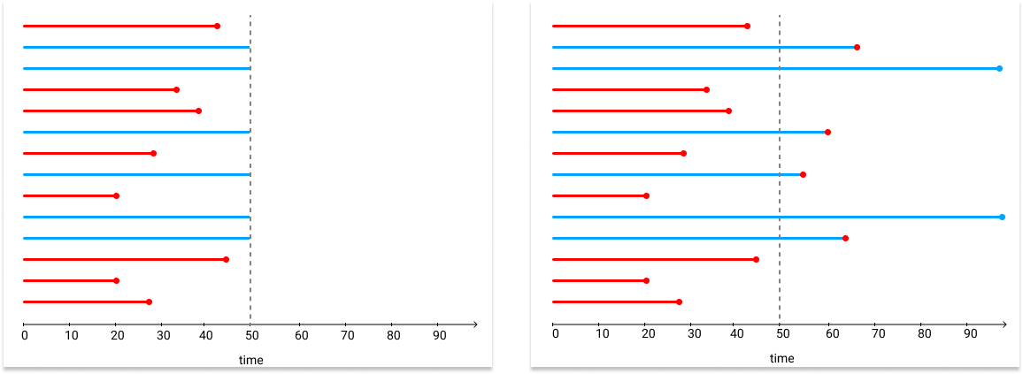
where the censoring time is at 50. Blue lines stand for the observations are still alive up to the censoring time, but some of them actually died after that. Red lines stand for the observations died before time 50, which means those death events are observed in the dataset.

Survival Analysis

Survival analysis was first developed by actuaries and medical professionals to predict survival rates based on censored data. Survival analysis can not only focus on medical industy, but many others.

There are several statistical approaches used to investigate the time it takes for an event of interest to occur. For example:

• Customer churn: duration is tenure, the event is churn;
• Machinery failure: duration is working time, the event is failure;
• Visitor conversion: duration is visiting time, the event is purchase.

In R, the may package used is survival. In Python, the most common package to use us called lifelines.

Kaplan-Meier Estimator

Kaplan-Meier Estimator is a non-parametric statistic used to estimate the survival function from lifetime data. The Kaplan-Meier Estimate defined as:

$\hat{S}(t) = \prod_{t_i \lt t} \frac{n_i - d_i}{n_i}$

where $d_i$ are the number of death events at time $t$ and $n_i$ is the number of subjects at risk of death just prior to time $t$.

Python Example

Here is an short example using lifelines package:

# load data
from lifelines.datasets import load_dd
data = load_dd()
data.head()

# load KaplanMeierFitter
from lifelines import KaplanMeierFitter
kmf = KaplanMeierFitter()

# define time and event columns
T = data["duration"]
E = data["observed"]

# fit data
kmf.fit(T, event_observed=E)

# plot survival curve
kmf.survival_function_.plot()
plt.title('Survival function of political regimes');

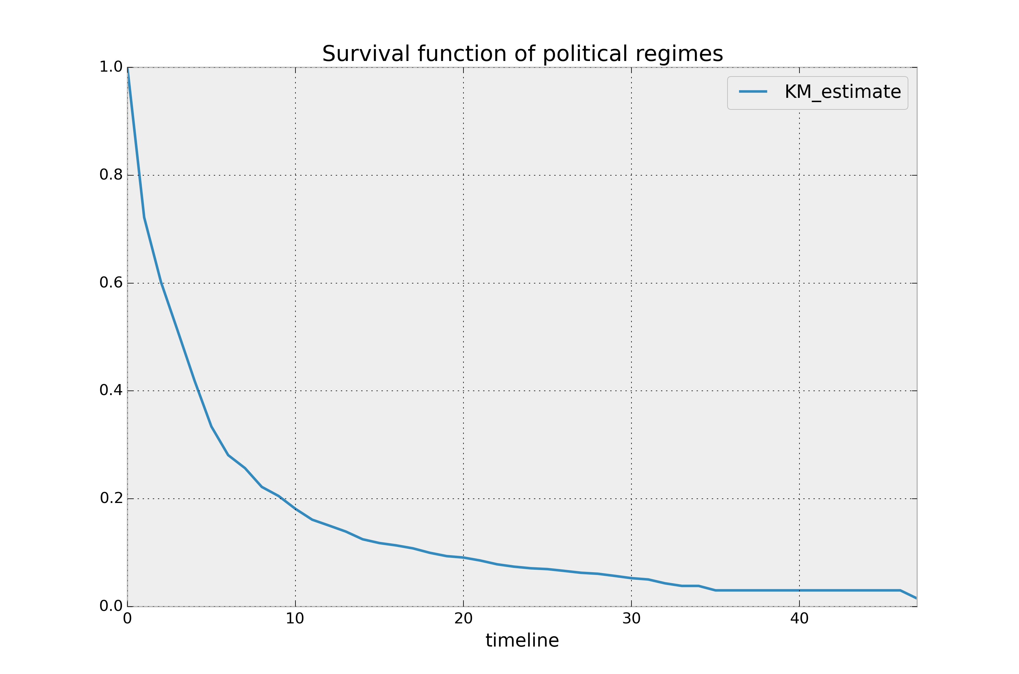
(source: lifelines)

This is an full example of using the Kaplan-Meier, results available in Jupyter notebook: survival_analysis/example_dd.ipynb

The Kaplan-Meier Estimator is an univariate model. It is not so helpful when many of the variables can affect the event differently. Further, the Kaplan-Meier Estimator can only incorporate on categorical variables.

Cox Proportional Hazard Model

To include multiple covariates in the model, we need to use some regression models in survival analysis. There are a few popular models in survival regression: Cox’s model, accelerated failure models, and Aalen’s additive model.

The Cox Proportional Hazards (CoxPH) model is the most common approach of examining the joint effects of multiple features on the survival time. The hazard function of Cox model is defined as:

$h_{i}(t)=h_{0}(t) e^{\beta_{1} x_{i 1}+\cdots+\beta_{p} x_{i p}}$

where $h_{0}(t)$ is the baseline hazard, $x_{i 1},...,x_{i p}$ are feature vectors, and $\beta_{1},...,\beta{p}$ are coefficients. The only time component is in the baseline hazard, $h_{0}(t)$. In the above product, the partial hazard is a time-invariant scalar factor that only increases or decreases the baseline hazard. Thus a changes in covariates will only increase or decrease the baseline hazard.

The major assumption of Cox model is that the ratio of the hazard event for any two observations remains constant over time:

$\frac{h_{i}(t)}{h_{j}(t)} = \frac{h_{0}(t) e^{\eta_{i}}}{h_{0}(t) e^{\eta_{j}}} = \frac{e^{\eta_{i}}}{e^{\eta_{j}}}$

where $i$ and $j$ are any two observations.

The Cox model is a semi-parametric model which mean it can take both numerical and categorical data. But categorical data requires to be preprocessed with one-hot encoding. For more information on how to use One-Hot encoding, check this post: Feature Engineering: Label Encoding & One-Hot Encoding.

Python Example

Here we use a numerical dataset in the lifelines package:

# import Cox model and load data
from lifelines import CoxPHFitter
from lifelines.datasets import load_rossi

# call dataset
rossi_dataset = load_rossi()

# call CoxPHFitter
cph = CoxPHFitter()

# fit data
cph.fit(rossi_dataset, duration_col='week', event_col='arrest', show_progress=True)

# print statistical summary
cph.print_summary()  # access the results using cph.summary

We metioned there is an assumption for Cox model. It can be tested by check_assumptions() method in lifelines package:

cph.check_assumptions()

Further, Cox model uses concordance-index as a way to measure the goodness of fit. Concordance-index (between 0 to 1) is a ranking statistic rather than an accuracy score for the prediction of actual results, and is defined as the ratio of the concordant pairs to the total comparable pairs:

• 0.5 is the expected result from random predictions,
• 1.0 is perfect concordance and,
• 0.0 is perfect anti-concordance (multiply predictions with -1 to get 1.0)

This is an full example of using the CoxPH model, results available in Jupyter notebook: survival_analysis/example_CoxPHFitter_with_rossi.ipynb

Survival Analysis in Machine Learning

There are several works about using survival analysis in machine learning and deep learning. Please check the packages for more information.

• DeepSurv: adaptively select covariates in Cox model.
• TFDeepSurv: TensorFlow version of DeepSurv with some improvements.
• LASSO for Cox: use LASSO for covariates selection in Cox model.
• ...

More examples about survival analysis and further topics are available at: https://github.com/huangyuzhang/cookbook/tree/master/survival_analysis/

References

• Davidson-Pilon, C., Kalderstam, J., Zivich, P., Kuhn, B., Fiore-Gartland, A., Moneda, L., . . .Rendeiro, A. F. (2019, August).Camdavidsonpilon/lifelines: v0.22.3 (late).Retrieved from https://doi.org/10.5281/zenodo.3364087 doi: 10.5281/zenodo.3364087
• Fox, J. (2002). Cox proportional-hazards regression for survival data. An R and S-PLUS companion to applied regression,2002.
• Simon, S. (2018).The Proportional Hazard Assumption in Cox Regression. The Anal-ysis Factor.
• Steck, H., Krishnapuram, B., Dehing-oberije, C., Lambin, P., & Raykar, V. C. (2008). Onranking in survival analysis: Bounds on the concordance index. InAdvances in neuralinformation processing systems(pp. 1209–1216).
• Ture, M., Tokatli, F., & Kurt, I. (2009). Using kaplan–meier analysis together with decisiontree methods (c&rt, chaid, quest, c4. 5 and id3) in determining recurrence-free survivalof breast cancer patients.Expert Systems with Applications,36(2), 2017–2026.